Urban Sprawl Data
Data and replication files for 'Causes of sprawl: A portrait from space'
by Marcy Burchfield, Henry G. Overman, Diego Puga, and Matthew A. Turner
This site distributes and documents the urban sprawl dataset created by Marcy Burchfield, Henry G. Overman, Diego Puga, and Matthew A. Turner and used in their article 'Causes of sprawl: A portrait from space', published in the Quarterly Journal of Economics 121(2), May 2006: 587-633, as well as the computer code required to replicate their results. Users of this dataset are asked to cite the Quarterly Journal of Economics article as the source. We would also appreciate it if you let us know the details of any paper in which you use the data by sending an email to Diego Puga (diego.puga@cemfi.es).
There are two main components in this dataset available at the following links. Documentation for the two components follows the links:
- The metropolitan-level sprawl data and computer code required to replicate the regressions in the article 'Causes of sprawl: A portrait from space'. These data and replication files, documented below, are available for download as a zip file. This contains the data in Stata and in ascii format, as well as a Stata do file that replicates the regressions and summary statistics in Table IV of the article:
sprawl_msa.zip(59 Kb) . - Supplementary land use and land cover data for three portions of the conterminous United States that are missing from the 1:250,000-scale Land Use and Land Cover GIRAS Data collected by U.S. Geological Survey (USGS) and distributed by the U.S. Environmental Protection Agency (EPA). These data, also documented below, are available for download as three zip files, each containing in shapefile format supplementary land use and land cover data for the missing portion of one 1:250,000 quadrangle:
- Albuquerque:
albunm_h.zip(1,596 Kb) . - Cedar City:
cedaut_h.zip(1,128 Kb) . - Tampa:
tampfl_h.zip(813 Kb) .
- Albuquerque:
Metropolitan-Level Sprawl Data
The article 'Causes of sprawl: A portrait from space' is concerned with a crucial aspect of sprawl, the scatteredness of development. We measure this aspect of sprawl as carefully as possible and study what causes differences across U.S. metropolitan areas in the extent to which urban development is sprawling or compact.
In order to be able to study detailed spatial patterns or urban development, we construct a new data set by merging high-altitude photographs from 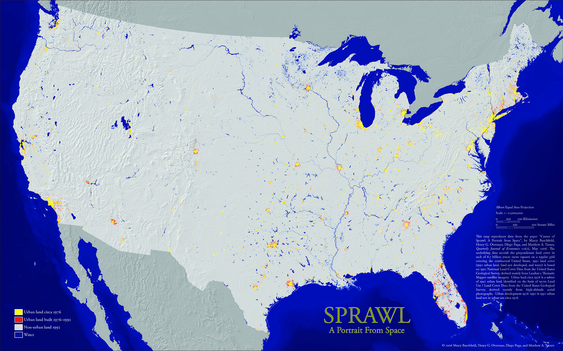 around 1976 with satellite images from 1992. From these data, described in some detail below, for units that are square cells of 30×30 meters, we know whether land was developed or not around 1976 and in 1992, as well as details about the type of developed or undeveloped land. Our data set consists of 8.7 billion such 30×30 meter cells for a grid covering the entire conterminous United States. A poster (11×17in) with a map based on these data showing urban development across the continental United States 1976-1992 is available as a pdf file
(4,276 Kb) by clicking on the thumbnail to the left of this paragraph.
around 1976 with satellite images from 1992. From these data, described in some detail below, for units that are square cells of 30×30 meters, we know whether land was developed or not around 1976 and in 1992, as well as details about the type of developed or undeveloped land. Our data set consists of 8.7 billion such 30×30 meter cells for a grid covering the entire conterminous United States. A poster (11×17in) with a map based on these data showing urban development across the continental United States 1976-1992 is available as a pdf file
(4,276 Kb) by clicking on the thumbnail to the left of this paragraph.
To measure the extent of sprawl, for each 30-meter cell of residential development, we calculate the percentage of open space in the immediate square kilometer. We then average across all residential development in each metropolitan area to compute an index of sprawl. For instance, to calculate a sprawl index for the new development that took place between 1976 and 1992 in each metropolitan area, we identify 30-meter cells that were not developed in 1976 but were subject to residential development between 1976 and 1992, calculate the percentage of land not developed by 1992 in the square kilometer containing each of these 30-meter cells, and average across all such newly developed cells in the metropolitan area. We also perform similar calculations to calculate a sprawl index for the stock of development in 1976 and in 1992. This provides a very intuitive index of sprawl: the percentage of undeveloped land in the square kilometer surrounding an average residential development.
The spatial units of observation in the metropolitan-level sprawl data are individual metropolitan areas (although, obviously, our calculations of the sprawl indices and various explanatory variables still need to use the full spatial resolution of our land use and land cover data). We use the Metropolitan Statistical Area and Consolidated Metropolitan Statistical Area definitions (New England County Metropolitan Area definitions for New England). Since these are county-based definitions, care is needed when measuring the initial characteristics of areas where new development might take place. This is particularly important in the western part of the country, where counties are sometimes very large and consequently metropolitan area boundaries are often drawn much less tightly around the developed portion of metropolitan areas than in the eastern part of the country. We therefore restrict calculations for geographical variables to the "urban fringe'', defined as those parts of the metropolitan area that were mostly undeveloped in 1976 but are located within 20 kilometers of areas that were mostly developed in 1976 (by mostly developed we mean areas where over 50 percent of the immediate square kilometer was developed in 1976). The choice of 20 kilometers as a threshold was guided by visual inspection of maps showing the evolution of land use in all metropolitan areas (a buffer of 20 kilometers around areas that were already mostly developed in 1976 includes 98 percent of 1976 residential development and 99 percent of subsequent residential development in metropolitan areas). Given that we isolate the urban fringe in this manner, it makes sense to start with fairly wide metropolitan area boundaries before we cut out areas far away from initial development. We therefore use 1999 definitions. We include all 275 metropolitan areas in the conterminous United States in our regressions.
The metropolitan-level sprawl data includes the following variables:
- msa: MSA/CMSA/NECMA FIPS code.
- msa_name: MSA/CMSA/NECMA name.
- sprawl_1976_92: Sprawl index for 1976-92 development. Percentage of land not developed by 1992 in the square kilometer around an average 1976-92 residential development in each metropolitan area.
- sprawl_1992: Sprawl index for 1992 development. Percentage of land not developed in the square kilometer around an average residential development in each metropolitan area in 1992.
- sprawl_1976: Sprawl index for 1976 development. Percentage of land not developed in the square kilometer around an average residential development in each metropolitan area in 1976.
- central_empl_1977: Centralized-sector employment 1977. For each metropolitan area, we use data from County Business Patterns, 1977 to calculate the share of employment in each three-digit SIC sector i, sMSA,i. For each sector, we know from Glaeser and Kahn (2001) the mean percentage of metropolitan area employment in that sector that is found within three miles of the central business district, s3,i (see their paper for details of the calculations). Our measure of centralization of employment is then calculated as ∑i sMSA,i × s3,i.
- streetcar_1902: Streetcar passengers per capita 1902. This is part of the segregation data from Cutler, Glaeser and Vigdor (1999).
- avg_dec_popgr1920_70: Mean decennial percentage population growth 1920-70. We calculate the percentage growth in each metropolitan area's population between each decennial census and the following one and calculate the mean over the period 1920-70. Constructing a historical series of population data for U.S. metropolitan areas on the basis of county population counts in each decennial census requires tracking changes in county boundaries over time. We did this using a revised version of the County Longitudinal Template of Horan and Hargis (1995) kindly provided to us by Vernon Henderson and Jordan Rappaport.
- sd_dec_popgr1920_70: Std. dev. decennial percentage population growth 1920-70. We calculate the percentage growth in each metropolitan area's population between each decennial census and the following one and calculate the standard deviation over the period 1920-70.
- pc_aquifer_fringe: Percentage of urban fringe overlaying aquifers. We use data from Principal Aquifers of the 48 Conterminous United States, Hawaii, Puerto Rico, and the us Virgin Islands, originally developed by the USGS to produce the maps printed in the Ground Water Atlas of the United States. This contains the shallowest principal aquifer at each point of the United States in a continuous geographical coverage. We exclude shallow sand and gravel aquifers since their high permeability and shallow depth to the water table makes them particularly susceptible to contamination from nitrates and other pollutants whose presence in sufficient quantity renders water unsuitable for human consumption
- pc_aquifer_msa: Percentage of MSA overlaying aquifers. Same as pc_aquifer_fringe, but for the entire metropolitan area.
- elevat_range_fringe: Elevation range in urban fringe (m.). We assemble a national elevation grid providing the elevation in meters of points 90 meters apart by merging and then reprojecting to an Albers Equal Area projection 922 separate elevation grids from the 1:250,000-scale Digital Elevation Models of the USGS, each of which provides 3-arc-second elevation data for an area of one by one degrees. The elevation range in urban fringe is the difference between the maximum and the minimum elevation in the urban fringe of each metropolitan area.
- elevat_range_msa: Elevation range in MSA (m.). Same as elevat_range_fringe, but for the entire metropolitan area.
- ruggedness_fringe: Terrain ruggedness index in urban fringe (m.). We use the same the national elevation grid providing the elevation in meters of points 90 meters apart as for elevat_range_fringe. Using these data, we calculate the terrain ruggedness index originally devised by Riley, DeGloria and Elliot (1999) to quantify topographic heterogeneity that can act either as concealment for prey or stalking cover for predators in wildlife habitats. Let er,cdenote elevation at the point located in row r and column c of a grid of elevation points. Then the terrain ruggedness index of Riley, DeGloria and Elliot (1999) at that point is calculated as ∑i=r-1i=r+1∑j=c-1j=c+1 (ei,j - er,c)2. The variable used in the regression is the average terrain ruggedness index of the urban fringe in each metropolitan area.
- ruggedness_msa: Terrain ruggedness index in MSA (m.). Same as ruggedness_fringe, but for the entire metropolitan area.
- cooling_dd: Mean cooling degree-days. Our weather variables are calculated from the climatic normals for individual weather stations 1961-1990 contained in the Climate Atlas of the United States. Cooling degrees on a given day are zero if the average temperature is below 65 °F (about 18 °C) and the degrees by which the average temperature exceeds 65 °F otherwise. Mean annual cooling degree days are computed by summing cooling degrees over all days in a year. We computed metropolitan area mean cooling degree days by averaging climatic normals over all reporting weather stations in each metropolitan area. For the four metropolitan areas that did not contain a reporting station, we averaged data from weather stations within 30 kilometers of the metropolitan area.
- heating_dd: Mean heating degree-days. Mean annual heating degree days are similarly calculated by summing degrees below 65 °F over all days in a year. Again, we computed metropolitan area mean heating degree days by averaging climatic normals over all reporting weather stations in each metropolitan area. For the four metropolitan areas that did not contain a reporting station, we averaged data from weather stations within 30 kilometers of the metropolitan area.
- pc_incorp_fringe: Percentage of urban fringe incorporated 1980. Computed using a digital representation of the municipal boundaries in effect at the time of the 1980 census obtained from GeoLytics.
- pc_incorp_msa: Percentage of MSA incorporated 1980. Same as pc_incorp_fringe, but for the entire metropolitan area.
- pc_transfers: Intergovernmental transfers as percentage of local revenues 1967. Percentage of local government revenue that were transfer payments from other levels of government in 1967, calculated with data from the County and City Data Book, 1972.
- rest_bars: Bars and restaurants per thousand people. Number of establishments classified as eating and drinking places (SIC 5810) in County Business Patterns, 1977.
- road_density: Major road density in urban fringe (m./ha.). Meters of major road (interstate, other limited access, divided highway, other U.S. highway, other state primary highway, state secondary highway, improved road, parallel highway, toll road) per hectare, calculated from USGS 1980 digital line graphs.
- popgr_1970_90: Percentage population growth 1970-90. Calculated using the same data as for avg_dec_popgr1920_70.
- herfindahl_incorp: Herfindahl index of incorporated place sizes. Computed using a digital representation of the municipal boundaries in effect at the time of the 1980 census obtained from GeoLytics.
- latitude: Latitude of the centroid of each metropolitan area.
- longitude: Longitude of the centroid of each metropolitan area.
- division: Census division.
This list includes all variables required to run the regressions in Table IV of the article 'Causes of sprawl: A portrait from space' plus several urban fringe variables re-calculated for the entire metropolitan area, in case these are useful for other purposes.
The metropolitan-level sprawl data is freely available for download from this site as a zip file: sprawl_msa.zip
(59 Kb) . This contains:
- The metropolitan-level data in Stata version 7 format:
sprawl_msa.dta. - The metropolitan-level data in comma-delimited ASCII format:
sprawl_msa.csv. - A Stata do file that re-creates the regressions and summary statistics contained in Table IV of the article 'Causes of sprawl: A portrait from space':
sprawl_regr.do. This has been tested to run in Stata versions 7, 8, and 9.
Supplementary Land Use and Land Cover Data
The sprawl indices used in the article 'Causes of sprawl: A portrait from space' were constructed from two fine-resolution data sets describing land cover and land use across the conterminous United States for the mid-1970s and the early 1990s.
The most recent data set, the 1992 National Land Cover Data classifies the land area circa 1992 into different land cover categories mainly on the basis of Landsat 5 Thematic Mapper satellite imagery. These data are the result of a collaboration between the U.S. Geological Survey (USGS) and the U.S. Environmental Protection Agency (EPA). The USGS makes them freely available for download as a set of 49 raster files (one for each state except Alaska and Hawaii and one for the District of Columbia) from http://edcftp.cr.usgs.gov/pub/data/landcover/states/ (see the metadata documentation for Massachusetts).
The earlier data set, the Land Use and Land Cover GIRAS Spatial Data, derives mainly from high-altitude aerial photographs taken mostly in the mid-1970s (1976 being the median and modal year). These data were collected by USGS and converted to ArcInfo format by the EPA. The EPA makes the data freely available for download as a set of 469 ArcInfo vector coverages (one for each 1:250,000-scale USGS quadrangle) from http://www.epa.gov/ngispgm3/spdata/EPAGIRAS/ (see the metadata documentation). An alternative version is available also from the EPA through their BASINS program from http://www.epa.gov/waterscience/basins/ (see the metadata documentation).
These digital versions of the 1970s Land Use and Land Cover GIRAS Spatial Data from 1:250,000-scale maps lack data for a thirty by sixty minute rectangle in the map for Albuquerque and also in the map for Cedar City and for a one degree by one degree square in the map for Tampa.
Fortunately, in addition to producing 1:250,000-scale maps (covering quadrangles of one degree by two degrees) for the conterminous United States, the USGS produced 1:100,000-scale maps (covering quadrangles of 30 minutes by 60 minutes) for some parts of the nation. For Albuquerque and Cedar City, the USGS had digitized data from the 1:100,000-scale maps corresponding exactly to the rectangles with missing data (Chaco Mesa in the case of Albuquerque, and Kanab in the case of Cedar City). We obtained the original digital data for these 1:100,000-scale maps from the USGS and processed them with the same computer code used by the EPA for the rest of the nation to completely fill the gaps. This involved:
- Downloading the GIRAS data for the 1:100,000-scale maps for Chaco Mesa and Kanab from http://edc.usgs.gov/geodata/.
- Gunzipping each downloaded file and adding delimiters to it with the command
dd if=land_use of=landuse ibs=8000 cbs=80 conv=unblock. - Converting the GIRAS file into an ArcInfo coverage using the girasarc2.aml Arc Macro Language script provided by the EPA with their distribution of the data.
- Tidying up the ArcInfo coverage using the girasneat.aml Arc Macro Language script provided by the EPA with their distribution of the data.
- Reprojecting to the North American Datum of 1983, converting the data into ArcInfo shapefile format, and adding metadata documentation.
For Tampa, the missing data were not available digitally but could be found in the corresponding 1:250,000-scale paper map distributed by the USGS. We obtained a copy from the University of Toronto Map Library and digitized this to the same format specifications as the rest of the data.
The 1970s land use and land cover data for these three areas (missing from the 1:250,000-scale Land Use and Land Cover GIRAS Data) are freely available from this site in ArcInfo shapefile format, zipped into one file per area:
- For the missing portion of the Albuquerque 1:250,000 quadrangle:
albunm_h.zip(1,596 Kb) . - For the missing portion of the Cedar City 1:250,000 quadrangle:
cedaut_h.zip(1,128 Kb) . - For the missing portion of the Tampa 1:250,000 quadrangle:
tampfl_h.zip(813 Kb) .
- The projection details for these three shapefiles are the following:
- Map projection: Albers Conical Equal Area
- Standard Parallel: 29.5
- Standard Parallel: 45.5
- Longitude of Central Meridian: -96.0
- Latitude of Projection Origin: 23.0
- Horizontal Datum: North American Datum 1983
- Ellipsoid: Geographic Reference System 80
- Semi-major Axis: 6378137
- Denominator of Flattening Ratio: 298.257
The land use and land cover codes (LUCODE attribute field) correspond to the same Anderson level 2 classification used in the USGS/EPA 1970s data. See the metadata documentation included with each shapefile for additional details.
Users interested in obtaining the same disaggregate data that served as the basis for the article 'Causes of sprawl: A portrait from space' will need three sets of files:
- The 49 raster files of the 1992 National Land Cover Data that the USGS makes freely available from http://edcftp.cr.usgs.gov/pub/data/landcover/states/.
- The 469 vector coverages of the 1970s Land Use and Land Cover GIRAS Spatial Data that the EPA makes freely available from http://www.epa.gov/ngispgm3/spdata/EPAGIRAS/.
- The three shapefiles for the portions of Albuquerque, Cedar City and Tampa missing from the 1970s Land Use and Land Cover GIRAS Spatial Data that are freely available from this site:
albunm_h.zip,cedaut_h.zipandtampfl_h.zip.
While there are many similarities between the 1970s and the 1990s data, there are a few important differences that users should be aware of.
First, the 1990s data are stored in raster format (assigning a code to each cell on a regular grid) while the 1970s data are stored in vector format (assigning a code and providing coordinates for irregular polygons). They also have different geographical projections. Thus, one needs to convert both data sets to a common projection and data model. For our analysis, we converted the 1970s data to the same projection and data model as the 1990s data, by breaking up each polygon into the 30-meter cells it contains.
The second difference is that the data are categorized using classifications with different degrees of detail. For our analysis, we worked with two urban codes that can be defined as aggregates of codes available in both years: residential; and commercial, industrial, and transportation networks.
The third and most important difference arises from some subtle, but relevant, differences in the thresholds used to classify an area as developed in the 1970s and in the 1990s data. Given this, we believe one should not compare the data directly. Instead, one can take advantage of the fact that, while land is often redeveloped, it is almost never undeveloped. At the national level, according to the U.S. Department of Agriculture's National Resource Inventory, less than 0.8% of developed land was converted from urban to non-urban uses over the 15-year period 1982-1997. With virtually no undevelopment taking place, we can base our analysis on the 1990s data and use the 1970s data to figure out whether each development that existed in 1992 was built before or after the 1970s. Thus, we define old development as land that was classified as urban in both the 1990s and 1970s. We define new development as land that was classified as urban in the 1990s, but was not urban in the 1970s. We also use the 1970s data to account for any conversion between residential and commercial uses.
Users interested in performing analysis at the level of metropolitan areas need not reproduce our aggregation procedure, and can work directly with the metropolitan-level data that we describe and make available above.
References
James R. Anderson, Ernest E. Hardy, John T. Roach, and Richard E. Witmer. 1976. A Land Use and Land Cover Classification System for Use with Remote Sensor Data. U.S. Geological Survey Professional Paper 964.
Burchfield, Marcy, Henry G. Overman, Diego Puga, and Matthew A. Turner. 2006. Causes of sprawl: A portrait from space. Quarterly Journal of Economics 121(2): 587-633.
Cutler, David M., Edward L. Glaeser, and Jacob L. Vigdor. 1999. The rise and decline of the American ghetto. Journal of Political Economy 107(3):455-506.
GeoLytics. 2000. CensusCD 1980, Version 2. East Brunswick, NJ: GeoLytics, Inc.
Glaeser, Edward L. and Matthew Kahn. 2001. Decentralized employment and the transformation of the American city. Brookings-Wharton Papers on Urban Affairs:1-47.
Horan, Patrick M. and Peggy G. Hargis. 1995. County Longitudinal Template, 1840-1990. Ann Arbor, MI: Inter-university Consortium for Political and Social Research (ICPSR 6576).
Riley, Shawn J., Stephen D. DeGloria, and Robert Elliot. 1999. A terrain ruggedness index that quantifies topographic heterogeneity. Intermountain Journal of Sciences 5(1-4):23-27.
U.S. Bureau of the Census. 1974. County and City Data Book, 1972. Ann Arbor, MI: Interuniversity Consortium for Political and Social Research (ICPSR 0061).
U.S. Bureau of the Census. 1999. County Business Patterns, 1977. Ann Arbor, MI: Interuniversity Consortium for Political and Social Research (ICPSR 8464).
U.S. Department of Agriculture. 2000. Summary Report: 1997 National Resources Inventory (revised December 2000). Washington, DC, and Ames, IA: United States Department of Agriculture, Natural Resources Conservation Service, and Statistical Laboratory Iowa State University.
U.S. Environmental Protection Agency. 1994. 1:250,000-scale Quadrangles of Landuse/Landcover GIRAS Spatial Data in the Conterminous United States. Washington, DC: United States Environmental Protection Agency, Office of Information Resources Management.
U.S. Geological Survey. 1990. Land Use and Land Cover Digital Data from 1:250,000- and 1:100,000-scale Maps: Data User Guide 4. Reston VA: United States Geological Survey.
U.S. Geological Survey. 1994. 1:250,000-scale Digital Elevation Models. Reston VA: United States Geological Survey.
U.S. Geological Survey. 2000. Ground Water Atlas of the United States. Reston VA: United States Geological Survey.
U.S. Geological Survey. 2003. Principal Aquifers of the 48 Conterminous United States, Hawaii, Puerto Rico, and the U.S. Virgin Islands. Madison WI: United States Geological Survey.
U.S. National Climatic Data Center. 2002. Climate Atlas of the United States, Version 2. Asheville, NC: United States National Climatic Data Center.
Vogelmann, James E., Stephen M. Howard, Limin Yang, Charles R. Larson, Bruce K. Wylie, and Nick Van Driel. 2001. Completion of the 1990s National Land Cover data set for the conterminous United States from Landsat Thematic Mapper data and ancillary data sources. Photogrammetric Engineering & Remote Sensing 67(6):650-684.